[TOC]
Keras 튜토리얼 (1)
ANN, DNN으로 MNIST 데이터 구분하기.
- 기본적인 개념은 알고있다는 전제하에 keras 문법 활용 레시피 위주로 적어본다.
- 완성된 코드는 여기에서 확인 가능하다.
1. ANN
1.0. 필요 라이브러리 import
from keras.models import Sequential
from keras.layers import Dense
from keras import losses

import numpy as np
from keras import datasets  # mnist
from keras.utils import np_utils

import matplotlib.pyplot as plt
import seaborn as sns

import os
os.environ["CUDA_DEVICE_ORDER"]="PCI_BUS_ID"
os.environ["CUDA_VISIBLE_DEVICES"]="2"

sns.set()
sns.set(font="D2coding")
1.1. Data확인
1.1.0. 데이터 로딩
# data 확인
(X_train, y_train), (X_test, y_test) = datasets.mnist.load_data()
print(X_train.shape)
print(y_train.shape)
print(X_test.shape)
print(y_test.shape)

## 결과
(60000, 28, 28)
(60000,)
(10000, 28, 28)
(10000,)
데이터의 차원은 28\(\times\)28차원짜리 60000개의 x와 그것의 label인 (60000,)개의 리스트가 존재한다.
1.1.1 데이터 확인
plt.figure(figsize=(6,12))

for i in range(6):
    n = np.random.randint(0, len(X_train))
    plt.subplot(320+1+i)
    plt.imshow(X_train[n])
    plt.title(y_train[n])

다음과 같이 손글씨 이미지(28\(\times\)28)과 그것의 label로 이루어져 있다.
1.2. 데이터 전처리
1.2.1. One hot encoding화(categorical화)
Y_train = np_utils.to_categorical(y_train)
Y_test = np_utils.to_categorical(y_test)

n = np.random.randint(0, 100)
print(y_train[n])
print(Y_train[n])

print(y_test[n])
print(Y_test[n])

## 결과
9
[0. 0. 0. 0. 0. 0. 0. 0. 0. 1.]
2
[0. 0. 1. 0. 0. 0. 0. 0. 0. 0.]
우리가 가진 y의 값을 one hot encoding형으로 바꾼다.
1.2.2. 선형으로 잇기
X_train = X_train.reshape(-1, X_train.shape[1]*X_train.shape[2])
X_test = X_test.reshape(-1, X_test.shape[1]*X_test.shape[2])
print(X_train.shape)
print(X_test.shape)

##
(60000, 784) # 28*28
(10000, 784)
28\(\times\)28차원을 1차원으로 늘려준다.
1.3. ANN 모델 생성
## Sequential을 상속받는 ANN
class ANN(Sequential):
    def __init__(self, input_dim, hidden_dim, output_dim):
        super().__init__()
        self.add(Dense(hidden_dim,
                       input_dim=input_dim,
                       activation="relu",
                       name="input_Layer") )
        self.add(Dense(output_dim, a
                       ctivation="softmax",
                       name="output_Layer"), )
        self.compile(loss=losses.categorical_crossentropy,
                     optimizer="adam", metrics=['acc'])


model.summary()

# 결과
_________________________________________________________________
Layer (type)                 Output Shape              Param #
=================================================================
input_Layer (Dense)          (None, 100)               78500
_________________________________________________________________
output_Layer (Dense)         (None, 10)                1010
=================================================================
Total params: 79,510
Trainable params: 79,510
Non-trainable params: 0
_________________________________________________________________
- input_dim의 갯수(우리는 28\(\times\)28)만큼 입력받고 출력이 hidden_dim인 1차 레이어와 출력이 10가지(우리의 결과값 0~9)를 가지는 1차 레이어를 가지는 심플한 ANN모델이다.
1.4. 모델 실행
1.4.1 input Data 정의 및 모델 생성
# input data 정의
input_dim = X_train.shape[1]
hidden_layer = 100
output_dim = Y_train.shape[1]

# 모델 생성
model = ANN(input_dim, hidden_layer, output_dim)
- Input_shape : 우리는 28$\times$28를 넣어준다. (-1, 784)
- hidden_layer : 우리가 원하는 은닉층 갯수를 넣어준다.
- output_dim : 우리는 0~9까지의 10가지를 구분하는 모델이므로 10으로 해준다.
1.4.2 모델 실행
history = model.fit(X_train, Y_train, epochs=10, batch_size=100, validation_split=0.2)
# 문제로 X_train을 넣고
# 정답으로 Y_train 으로 확인을 하며
# 한번에 100개의 이미지를 가져와서 검증을 하며
# 10회의 반복문으로 한다.
# X_train의 갯수중 20%는 검증셋으로 한다.
1.4.3 모델 검정
loss, accuracy = model.evaluate(X_test, Y_test, batch_size=100)

print("Test Loss\t:\t{:2.4f}".format(loss))
print("Test Accuracy\t:\t{:2.4f}".format(accuracy))

# 결과
10000/10000 [==============================] - 0s 14us/step
Test Loss	    :	0.0761
Test Accuracy	:	0.9767
- 우리가 만든 검증셋인 X_test와 Y_test로 모델 검정을 한다.
- loss는 0.0761, 정확도는 97%정도가 나왔다.
1.4.4 결과 그래프
h = pd.DataFrame(history.history)

ax = h.plot(x="index", y=["loss", "val_loss"])
ax.set_ylabel("loss")
ax2 = ax.twinx()
ax2.set_ylabel("acc")
h.plot(x="index", y=["acc", "val_acc"], ax=ax2, colormap='viridis',)
plt.grid(False)
plt.show()
1.4.5 결과 확인
plt.figure(figsize=(6,12))

for i in range(6):
    n = np.random.randint(0, len(X_test))
    plt.subplot(320+1+i)
    plt.imshow(X_test[n].reshape(28, 28))
    plt.title("R:{}, P:{}".format(y_test[n], np.argmax(yhat_test[n])) )

- (1,0) 번째는 묘하게 생겨서 틀렸지만 정확도 약 97%의 분류기를 완성하였다.
2. DNN
ANN과 전처리단계는 같다
2.3. DNN 모델 생성
class DNN(Sequential):
    def __init__(self, input_dim, hidden_dim, output_dim, depth=5):
        super().__init__()
        self.add(Dense(hidden_dim, input_dim=input_dim, activation="relu", name="input_Layer") )
        for x in range(depth):
            self.add(Dense(hidden_dim, activation="relu", name="hidden_layer_{:02}".format(x)))
        self.add(Dense(output_dim, activation="softmax", name="output_Layer"), )
        self.compile(loss=losses.categorical_crossentropy,
                     optimizer="adam", metrics=['acc'])
- 위의 ANN에서 히든층을 늘렸다. (기본 5층)
2.4 모델 실행
실행은 역시 위의 ANN과 같다. 결과만 표시한다.
2.4.1 모델 생성
# input data 정의
input_dim = X_train.shape[1]
hidden_layer = 100
output_dim = Y_train.shape[1]

# 모델 생성
dnn = DNN(input_dim, hidden_layer, output_dim, depth=20)

dnn.summary()

# 결과
_________________________________________________________________
Layer (type)                 Output Shape              Param #
=================================================================
input_Layer (Dense)          (None, 100)               78500
_________________________________________________________________
hidden_layer_00 (Dense)      (None, 100)               10100
_________________________________________________________________
hidden_layer_01 (Dense)      (None, 100)               10100
_________________________________________________________________
hidden_layer_02 (Dense)      (None, 100)               10100
_________________________________________________________________
hidden_layer_03 (Dense)      (None, 100)               10100
_________________________________________________________________
hidden_layer_04 (Dense)      (None, 100)               10100
_________________________________________________________________
hidden_layer_05 (Dense)      (None, 100)               10100
_________________________________________________________________
hidden_layer_06 (Dense)      (None, 100)               10100
_________________________________________________________________
hidden_layer_07 (Dense)      (None, 100)               10100
_________________________________________________________________
hidden_layer_08 (Dense)      (None, 100)               10100
_________________________________________________________________
hidden_layer_09 (Dense)      (None, 100)               10100
_________________________________________________________________
hidden_layer_10 (Dense)      (None, 100)               10100
_________________________________________________________________
hidden_layer_11 (Dense)      (None, 100)               10100
_________________________________________________________________
hidden_layer_12 (Dense)      (None, 100)               10100
_________________________________________________________________
hidden_layer_13 (Dense)      (None, 100)               10100
_________________________________________________________________
hidden_layer_14 (Dense)      (None, 100)               10100
_________________________________________________________________
hidden_layer_15 (Dense)      (None, 100)               10100
_________________________________________________________________
hidden_layer_16 (Dense)      (None, 100)               10100
_________________________________________________________________
hidden_layer_17 (Dense)      (None, 100)               10100
_________________________________________________________________
hidden_layer_18 (Dense)      (None, 100)               10100
_________________________________________________________________
hidden_layer_19 (Dense)      (None, 100)               10100
_________________________________________________________________
output_Layer (Dense)         (None, 10)                1010
=================================================================
Total params: 281,510
Trainable params: 281,510
Non-trainable params: 0
_________________________________________________________________
2.4.2 모델 실행
history = dnn.fit(X_train, Y_train, epochs=10, batch_size=100, validation_split=0.2)

# 결과
Train on 48000 samples, validate on 12000 samples
Epoch 1/10
48000/48000 [==============================] - 8s 170us/step - loss: 0.9352 - acc: 0.6524 - val_loss: 0.3273 - val_acc: 0.9017
Epoch 2/10
48000/48000 [==============================] - 7s 143us/step - loss: 0.2967 - acc: 0.9215 - val_loss: 0.2507 - val_acc: 0.9321
....
2.4.3 모델 검정
loss, accuracy = dnn.evaluate(X_test, Y_test, batch_size=100)
print("Test Loss\t:\t{:2.4f}".format(loss))
print("Test Accuracy\t:\t{:2.4f}".format(accuracy))

# 결과
10000/10000 [==============================] - 0s 20us/step
Test Loss	:	0.1129
Test Accuracy	:	0.9738
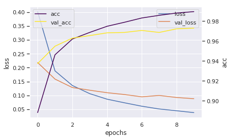
2.4.4 결과 그래프
h = pd.DataFrame(history.history)
h = h.reset_index()

ax = h.plot(x="index", y=["loss", "val_loss"])
ax.set_ylabel("loss")
ax2 = ax.twinx()
ax2.set_ylabel("acc")
h.plot(x="index", y=["acc", "val_acc"], ax=ax2, colormap='viridis',)
ax.set_xlabel("epochs")
plt.grid(False)

plt.show()

2.4.5 결과 확인
yhat_test = model.predict(X_test, batch_size=32)

plt.figure(figsize=(6,12))

for i in range(6):
    n = np.random.randint(0, len(X_test))
    plt.subplot(320+1+i)
    plt.imshow(X_test[n].reshape(28, 28))
    plt.title("R:{}, P:{}".format(y_test[n], np.argmax(yhat_test[n])) )
